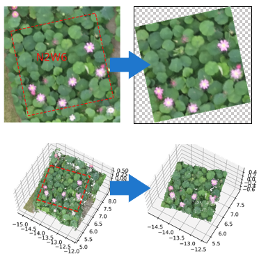
Crop DOM/DSM/PCD by ROI
Using region of interest (ROI, e.g. plot boundary), cropping each of them from large digital orthomosaic (DOM), digital surface model (DSM), and point cloud of whole field, without using any GIS or point cloud processing software.
Package and data prepare.
The easiest way to import easyidp package and using the demo exmaple is:
[1]:
import easyidp as idp

lotus = idp.data.Lotus()
If you run for the first time, it will download 3.3GB dataset automatically from Google Drive, please refer to Data for more details.
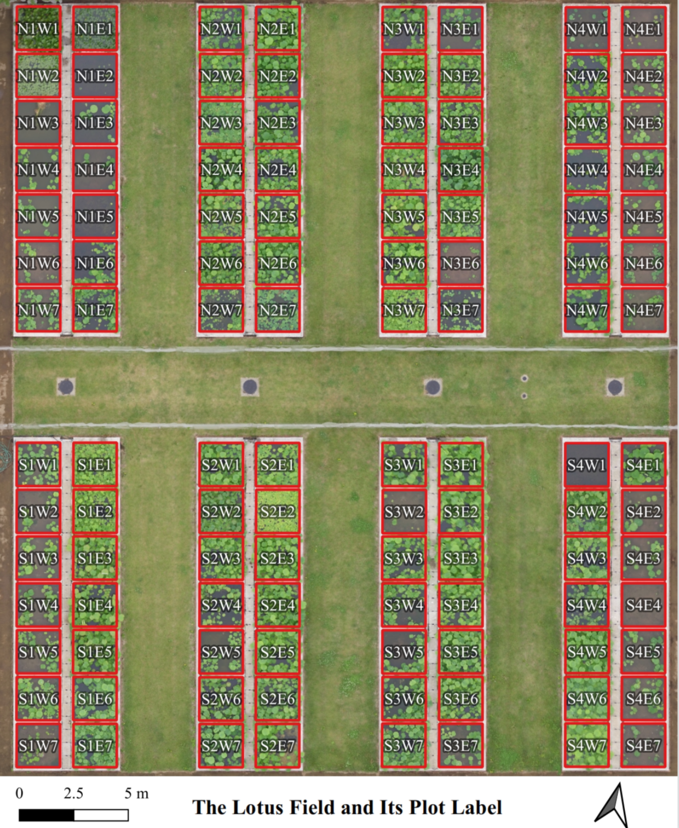
Read ROI from shapefile
The following code will load and open the plot boundary shapefile in the Lotus Dataset, the shp file looks like (red polygons):
[2]:
roi = idp.ROI(lotus.shp, name_field='plot_id')
[shp][proj] Use projection [WGS 84] for loaded shapefile [plots.shp]
Read shapefile [plots.shp]: 100%|██████████| 112/112 [00:00<00:00, 2347.62it/s]
[3]:
roi
[3]:
<easyidp.ROI> with 112 items
[0]     N1W1
array([[139.54052962,  35.73475194],
       [139.54055106,  35.73475596],
       [139.54055592,  35.73473843],
       [139.54053438,  35.73473446],
       [139.54052962,  35.73475194]])
[1]     N1W2
array([[139.54053488,  35.73473289],
       [139.54055632,  35.73473691],
       [139.54056118,  35.73471937],
       [139.54053963,  35.73471541],
       [139.54053488,  35.73473289]])
...
[110]   S4E6
array([[139.54090456,  35.73453742],
       [139.540926  ,  35.73454144],
       [139.54093086,  35.7345239 ],
       [139.54090932,  35.73451994],
       [139.54090456,  35.73453742]])
[111]   S4E7
array([[139.54090986,  35.73451856],
       [139.54093129,  35.73452258],
       [139.54093616,  35.73450504],
       [139.54091461,  35.73450107],
       [139.54090986,  35.73451856]])
See also
For more details about the parameter when loading shapefile, please refer to Load ROI from shapefile, or python API easyidp.ROI, and easyidp.shp.read_shp.
Read and crop geotiff (DOM/DSM)
First, open the DOM geotiff file by:
[4]:
lotus.metashape.dom
[4]:
PosixPath('/Users/hwang/Library/Application Support/easyidp.data/2017_tanashi_lotus/170531.Lotus.outputs/170531.Lotus_dom.tif')
[5]:
dom = idp.GeoTiff(lotus.metashape.dom)
See also
The GeoTiff is easyidp defined class contains several required information. Please check python API easyidp.GeoTiff for more information
However, in this case, the ROI and GeoTiff do not share the same geo-coordinate:
[6]:
print("ROI.CRS: ", roi.crs.name, "\nDOM.CRS: ", dom.crs.name)
ROI.CRS:  WGS 84
DOM.CRS:  WGS 84 / UTM zone 54N
Hence need to transform the ROI to the same CRS as GeoTiff, for more details please refer Load ROI from shapefile
[7]:
roi.change_crs(dom.crs)
Then using the following function to crop each ROI (plot) from whole field GeoTIff:
[8]:
dom_parts = roi.crop(dom)
Crop roi from geotiff [170531.Lotus_dom.tif]: 100%|██████████| 112/112 [00:03<00:00, 30.07it/s]
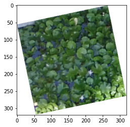
The output dom_parts is a dictionary, using plot label as keys and cropped imarray as values:
[9]:
import matplotlib.pyplot as plt
[10]:
plt.imshow(dom_parts['N1W1'])
[10]:
<matplotlib.image.AxesImage at 0x7fbf288812e0>
It you want to save the cropped GeoTiff, please pass the save_folder parameter when cropping
>>> dom_parts = roi.crop(dom, save_folder=r"expected\save\folder")
It will save all cropped sections to GeoTiff files with geo-offset (you can overlap the cropped DOM almost perfectly on the original DOM)
Future work
Currently can not just save the single output dom_parts["N1W1"] to standard GeoTiff file with correct geo-position without previoud save_folder batch saving, but in the future will support save such file directly via dom_part["N1W1"].save("path\to\save\N1W1.tif")
The step to crop DSM is the same as DOM, ignored here.
Read and crop point cloud
The point cloud also use the same process like GeoTIff
See also
The PointCloud is easyidp defined class contains several required information. Please check python API easyidp.PointCloud for more information
[11]:
pcd = idp.PointCloud(lotus.metashape.pcd)
Check the point cloud values:
[12]:
pcd
[12]:
                   x            y        z  r    g    b        nx      ny      nz
       0  368016.142  3955509.827   94.017  129  132  147  nodata  nodata  nodata
       1  368016.142  3955509.827   94.017  129  132  147  nodata  nodata  nodata
       2  368016.142  3955509.827   94.017  129  132  147  nodata  nodata  nodata
     ...     ...          ...      ...      ...  ...  ...     ...     ...     ...
10158190  368056.169  3955481.725   97.425  174  163  149  nodata  nodata  nodata
10158191  368056.51   3955481.904   97.44   166  153  139  nodata  nodata  nodata
10158192  368056.538  3955481.486   97.447  97   112  72   nodata  nodata  nodata
And cropping:
Caution
Please ensure the same CRS between ROI and PointCloud.
[13]:
pcd_parts = roi.crop(pcd)
Crop roi from point cloud [170531.Lotus.laz]: 100%|██████████| 112/112 [00:30<00:00, 3.61it/s]
The output pcd_parts is a dictionary, using plot label as keys and cropped point cloud as values:
[14]:
pcd_parts["N1W1"]
[14]:
                x            y        z  r       g       b           nx      ny      nz
    0  368017.889  3955510.812   97.214  nodata  nodata  nodata  nodata  nodata  nodata
    1  368017.888  3955510.8     97.218  nodata  nodata  nodata  nodata  nodata  nodata
    2  368017.897  3955510.964   97.22   nodata  nodata  nodata  nodata  nodata  nodata
  ...     ...          ...      ...      ...     ...     ...        ...     ...     ...
35745  368020.003  3955509.546   97.558  nodata  nodata  nodata  nodata  nodata  nodata
35746  368020.046  3955509.665   97.436  nodata  nodata  nodata  nodata  nodata  nodata
35747  368019.914  3955509.974   97.444  nodata  nodata  nodata  nodata  nodata  nodata
Similarly, you can pass the save_folder parameter to save the cropped point cloud
>>> pcd_parts = roi.crop(pcd, save_folder=r"expected\save\folder")
Or your can save just one point cloud by:
>>> pcd_part["N1W1"].save(r"path\to\save\N1W1.ply")