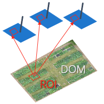
Backward Projection
这个例子解释了如何使用 EasyIDP 在原始无人机图像上找到 ROI 的对应位置。
包和数据准备
导入 easyidp 包的最常见方式是:
[1]:
import easyidp as idp

lotus = idp.data.Lotus()
如果您是第一次运行,它将自动从 Google Drive 下载 3.3GB 的数据集,请参考 Data 了解更多详情。
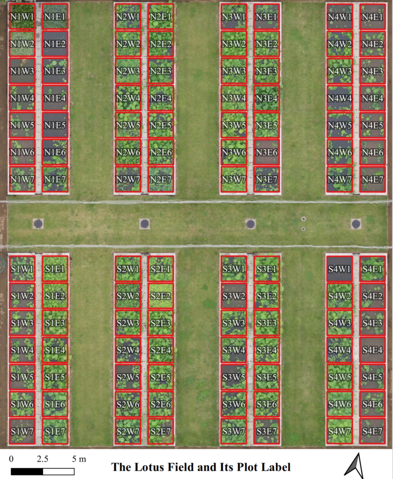
从 Shapefile 读取 ROI
然后打开 shapefile plot.shp,shp 文件看起来像这样(红色多边形):
[2]:
roi = idp.ROI(lotus.shp, name_field='plot_id')
[shp][proj] Use projection [WGS 84] for loaded shapefile [plots.shp]
Read shapefile [plots.shp]: 100%|██████████| 112/112 [00:00<00:00, 2406.33it/s]
然后检查它是否按预期加载:
[3]:
roi
[3]:
<easyidp.ROI> with 112 items
[0]     N1W1
array([[139.54052962,  35.73475194],
       [139.54055106,  35.73475596],
       [139.54055592,  35.73473843],
       [139.54053438,  35.73473446],
       [139.54052962,  35.73475194]])
[1]     N1W2
array([[139.54053488,  35.73473289],
       [139.54055632,  35.73473691],
       [139.54056118,  35.73471937],
       [139.54053963,  35.73471541],
       [139.54053488,  35.73473289]])
...
[110]   S4E6
array([[139.54090456,  35.73453742],
       [139.540926  ,  35.73454144],
       [139.54093086,  35.7345239 ],
       [139.54090932,  35.73451994],
       [139.54090456,  35.73453742]])
[111]   S4E7
array([[139.54090986,  35.73451856],
       [139.54093129,  35.73452258],
       [139.54093616,  35.73450504],
       [139.54091461,  35.73450107],
       [139.54090986,  35.73451856]])
从 DSM 获取高度(z)值
shapefile 中的 ROI 只有 2D 坐标,然而,要进行逆向投影,ROI 应该是 3D 坐标,缺失的高度值可以从 DSM 获取。
未来工作
未来将支持从点云获取 Z 值,在这种情况下,如果只需要逆向投影(在原始图像上进行图像分析而不是低质量的 geotiff),3D 重建可以在制作密集点云时停止,无需运行后续的 DOM 和 DSM 步骤。
[4]:
roi.get_z_from_dsm(lotus.metashape.dsm)
Read z values of roi from DSM [170531.Lotus_dsm.tif]: 100%|██████████| 112/112 [00:01<00:00, 100.17it/s]
并检查 ROI 的值
[5]:
roi
[5]:
<easyidp.ROI> with 112 items
[0]     N1W1
array([[ 368017.7565143 , 3955511.08102276,      97.39836121],
       [ 368019.70190232, 3955511.49811902,      97.39836121],
       [ 368020.11263046, 3955509.54636219,      97.39836121],
       [ 368018.15769062, 3955509.13563382,      97.39836121],
       [ 368017.7565143 , 3955511.08102276,      97.39836121]])
[1]     N1W2
array([[ 368018.20042946, 3955508.96051697,      97.31330109],
       [ 368020.14581791, 3955509.37761334,      97.31330109],
       [ 368020.55654627, 3955507.42585654,      97.31330109],
       [ 368018.601606  , 3955507.01512806,      97.31330109],
       [ 368018.20042946, 3955508.96051697,      97.31330109]])
...
[110]   S4E6
array([[ 368051.31139629, 3955486.78103425,      97.61438751],
       [ 368053.25678767, 3955487.19813795,      97.61438751],
       [ 368053.66752456, 3955485.24638299,      97.61438751],
       [ 368051.71258131, 3955484.83564713,      97.61438751],
       [ 368051.31139629, 3955486.78103425,      97.61438751]])
[111]   S4E7
array([[ 368051.75902187, 3955484.68169527,      97.59178925],
       [ 368053.70441367, 3955485.09879908,      97.59178925],
       [ 368054.11515079, 3955483.14704415,      97.59178925],
       [ 368052.16020711, 3955482.73630818,      97.59178925],
       [ 368051.75902187, 3955484.68169527,      97.59178925]])
我们可以注意到,roi 的 x 和 y 值也发生了变化。因为 ROI shp 地理坐标是 EPSG::4326,而 DSM 是 EPSG::32654。
另见
有关此功能控制的更多详细信息,请参考 从 DSM 获取高度(z)值
Read 3D reconstuction project and backward projection
对于 metashape 项目:
[6]:
ms = idp.Metashape(lotus.metashape.project, chunk_id=0)
对于 pix4d 项目:
[7]:
p4d = idp.Pix4D(project_path=lotus.pix4d.project,
                raw_img_folder=lotus.photo,
                param_folder=lotus.pix4d.param)
And then do the backward projection by:
[8]:
img_dict_ms = roi.back2raw(ms)
img_dict_p4d = roi.back2raw(p4d)
Backward roi to raw images: 100%|██████████| 112/112 [00:01<00:00, 56.75it/s]
Backward roi to raw images: 100%|██████████| 112/112 [00:01<00:00, 79.72it/s]
或
>>> img_dict_ms = ms.back2raw(roi)
>>> img_dict_p4d = p4d.back2raw(roi)
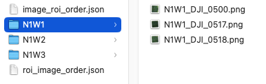
注意
您可以通过以下方式将结果(json 和裁剪的 png)保存到指定文件夹:
img_dict_sort = roi.back2raw(ms, ..., save_folder="folder_to_save")
并将在文件夹中获得以下结果:
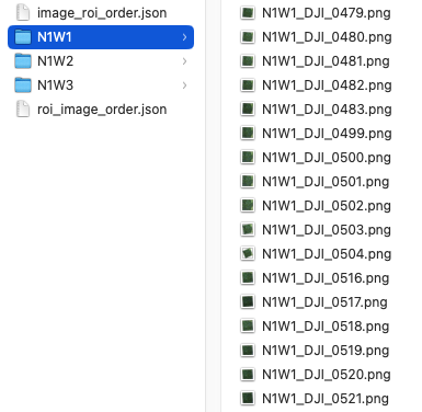
输出 img_dict 的结构是两层字典。第一层是 roi id,第二层是图像名称 (out_dict['roi_id']['image_name'])。
You can find all available images with specified roi (plot) (e.g. roi named ‘N1W1’) by:
>>> img_dict_ms['N1W1']
{'DJI_0479': array([[  43.91987253, 1247.04066872],
                    [  69.0221046 ,  972.89938018],
                    [ 353.25370817,  993.30409359],
                    [ 328.10701394, 1267.40353364],
                    [  43.91987253, 1247.04066872]]),
 'DJI_0480': array([[ 655.3678591 , 1273.01418098],
                    [ 681.18303761,  996.4866665 ],
                    [ 965.60719523, 1019.55346144],
                    [ 939.89408896, 1296.05588162],
                    [ 655.3678591 , 1273.01418098]]),
...
}
For example, find the roi named ‘N1W1’ on image ‘IMG_3457’ by:
[9]:
img_dict_ms["N1W1"]['DJI_0479']
[9]:
array([[  43.91987253, 1247.04066872],
       [  69.0221046 ,  972.89938018],
       [ 353.25370817,  993.30409359],
       [ 328.10701394, 1267.40353364],
       [  43.91987253, 1247.04066872]])
这是图像像素上 roi 的 2D 坐标
The recommended ‘for loops’ for itering items:
for roi_id, img_dict in out_dict.items():
    # roi_id = 'N1W1'
    # img_dict = out_dict[roi_id]
    for img_name, coords in img_dict.items():
        # img_name = "IMG_3457"
        # coords = out_dict[roi_id][img_name]
        print(coords)
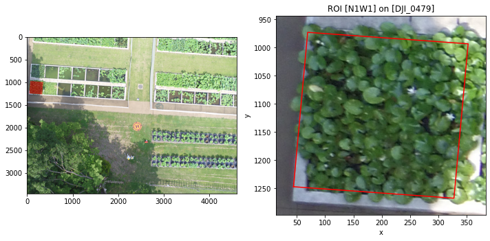
预览结果:
[10]:
ms.show_roi_on_img(img_dict_ms, "N1W1", "DJI_0479")
<Figure size 432x288 with 0 Axes>
或检查所有结果:
[11]:
ms.show_roi_on_img(img_dict_ms, "N1W1")
Reading image files for plotting: 100%|██████████| 17/17 [00:05<00:00, 2.88it/s]
Image data loaded, drawing figures, this may cost a few seconds...
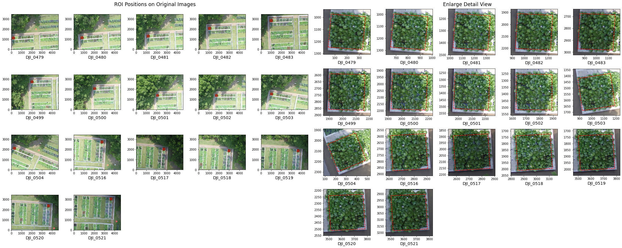
<Figure size 432x288 with 0 Axes>
推荐使用 ms.show_roi_on_img(..., save_as="preview_all.png") 保存到本地磁盘并检查清晰图像。
找到最佳逆向图像
您可以注意到,对于每个 ROI,它将逆向投影到几个原始图像:
[12]:
len(img_dict_ms["N1W1"])
[12]:
17
如何找到最佳的 3 或 5 张图像?在这里您可以计算图像到 ROI 的距离,这里我们假设距离越短越好(理想情况下,无人机图像刚好在 ROI 区域上方,ROI 位于图像中心)。
[13]:
img_dict_sort = ms.sort_img_by_distance(
    img_dict_ms, roi,
    distance_thresh=10,  # distance threshold is 2m
    num=3   # only keep 3 closest images
)
Getting photo positions: 100%|██████████| 151/151 [00:01<00:00, 126.79it/s]
Filter by distance to ROI: 100%|██████████| 112/112 [00:00<00:00, 1404.14it/s]
注意
您可以通过以下方式将结果(json 和裁剪的 png)保存到指定文件夹:
img_dict_sort = ms.sort_img_by_distance(..., save_folder="folder_to_save")
并将在文件夹中获得以下结果:
[14]:
img_dict_sort["N1W1"]
[14]:
{'DJI_0500': array([[1922.56317403, 2186.55026212],
        [1931.87582434, 1925.40596027],
        [2192.1757749 , 1934.43920442],
        [2182.74834419, 2195.88054775],
        [1922.56317403, 2186.55026212]]),
 'DJI_0517': array([[2865.83794784, 2151.98114332],
        [2592.43855364, 2169.39562183],
        [2574.82262634, 1895.17496101],
        [2848.48455635, 1878.83422193],
        [2865.83794784, 2151.98114332]]),
 'DJI_0501': array([[1964.74098137, 1514.46208287],
        [1974.95313868, 1258.05047894],
        [2233.01889145, 1269.92769931],
        [2222.63045448, 1526.62893437],
        [1964.74098137, 1514.46208287]])}
Here is the best 3 image that match “distance from ROI to image” < 10m, and the first one is the closest.
检查结果:
[15]:
ms.show_roi_on_img(img_dict_ms, "N1W1", "DJI_0500")
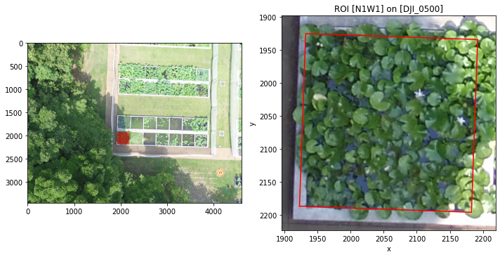
<Figure size 432x288 with 0 Axes>
或检查所有结果:
[16]:
ms.show_roi_on_img(img_dict_sort, "N1W1")
Reading image files for plotting: 100%|██████████| 3/3 [00:00<00:00, 3.12it/s]
Image data loaded, drawing figures, this may cost a few seconds...
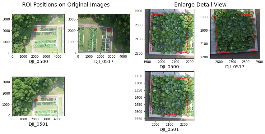
<Figure size 432x288 with 0 Axes>
推荐使用 ms.show_roi_on_img(..., save_as="preview_all.png") 保存到本地磁盘并检查清晰图像。